#Intuitive Explanation for Principle Component Analysis (PCA), in Six Minutes.

Principle Component Analysis (PCA) is arguably a very difficult-to-understand topic for beginners in machine learning. Here, I will try my best to intuitively explain what it is, how the algorithm does what it does. This post assumes you have very basic knowledge of Linear Algebra like matrix multiplication, and vectors.

#What is PCA?

PCA is a dimensionality-reduction technique used to make large datasets with hundreds of thousands of features into smaller datasets with fewer features while retaining as much information about the dataset as possible.

A perfect example would be:

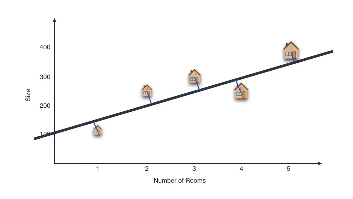
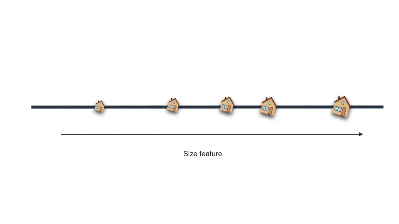
If we project the houses on the black line, we would get something like this:

So we need to reduce that projection error (the magnitude of blue lines) in order to retain maximum information.

#Prerequisites to understanding the PCA Algorithm.

I will explain some concepts intuitively in order for you to understand the algorithm better.

#Mean

Mean of any dataset refers to the equilibrium of the dataset. Imagine a rod on which balls are placed at some distance x from the wall:

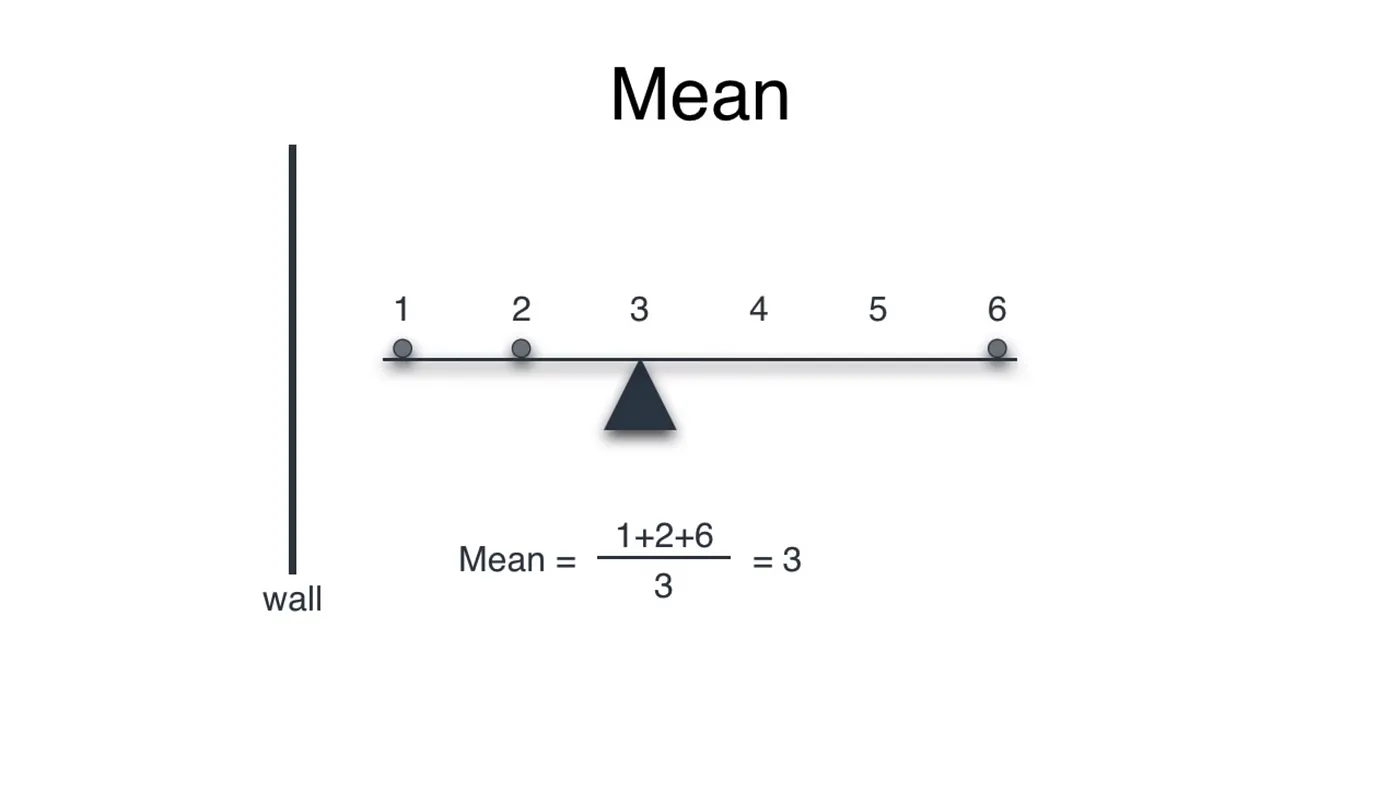
Summing the distance of the balls from the wall and dividing by the number of balls results the point of equilibrium, where a pivot would balance the rod.

#Variance

Mean tells us about the equilibrium of the dataset, variance is a metric that tells us about the spread of dataset from its mean. In 1-dimensional dataset, variance can be illustrated as:

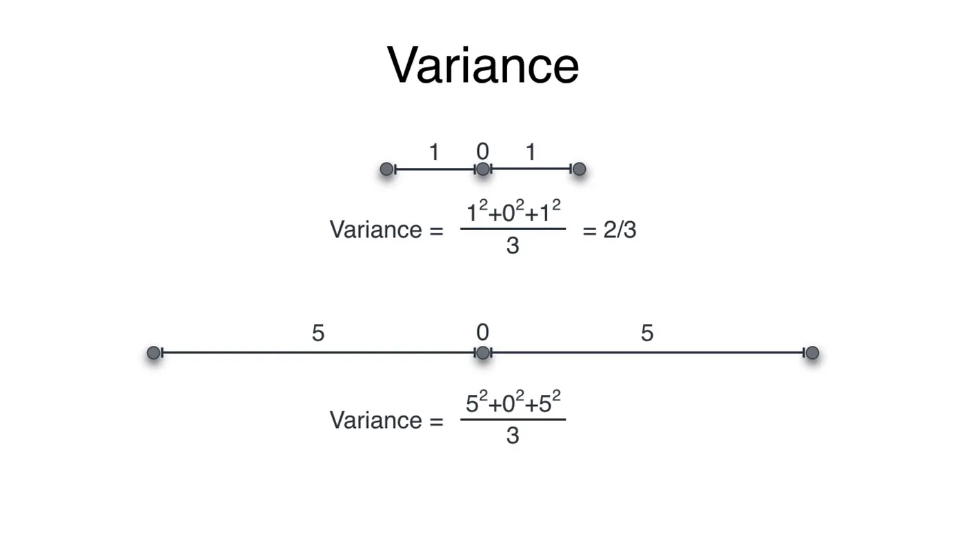
We take the square of each distance so we do not get any negative values!

#Covariance

In two and higher dimensional two very different datasets could have same variance, leading to misinterpretations of data. For example, both the datasets below have the same variance even though they are entirely different.

Covariance depicts the correlation of dataset. It is a quantity describing the variance as well as the direction of the spread. This will help us distinguish between the above two datasets.

The covariance matrix is a linear transformation that transforms given data into another shape. We will see that later. In 2D, this matrix is (2 x 2).

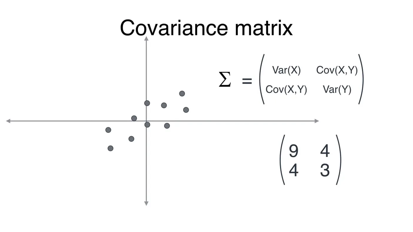
For the dataset in the example above, after inserting values, a rough estimate of the covariance matrix would be the one shown. To understand the use of this matrix we first need to understand linear transformations.

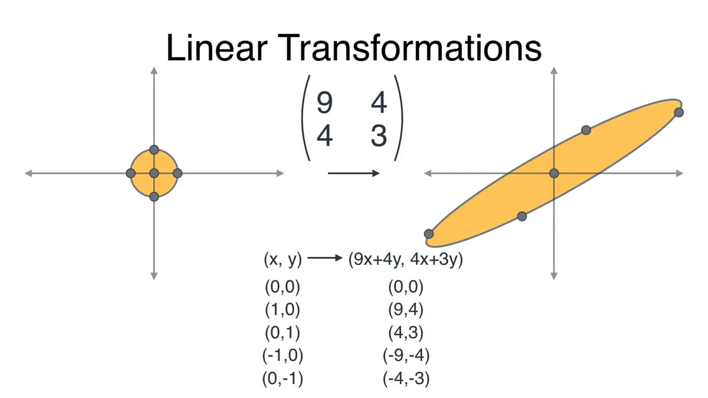
A linear transformation is a mapping that transforms any point in the 2D plane to another point in the same plane by using a transformation matrix.

Back to our example, the covariance matrix is our transformation matrix. A unit circle would be transformed into an ellipse by the covariance matrix (using matrix multiplication) as shown below.

This transformation gives us two very special vectors — the eigenvectors.

These eigenvectors are special because they are not affected by the transformation (their direction remains the same), they are only increased in magnitude. Below are the two vectors in red and teal color.

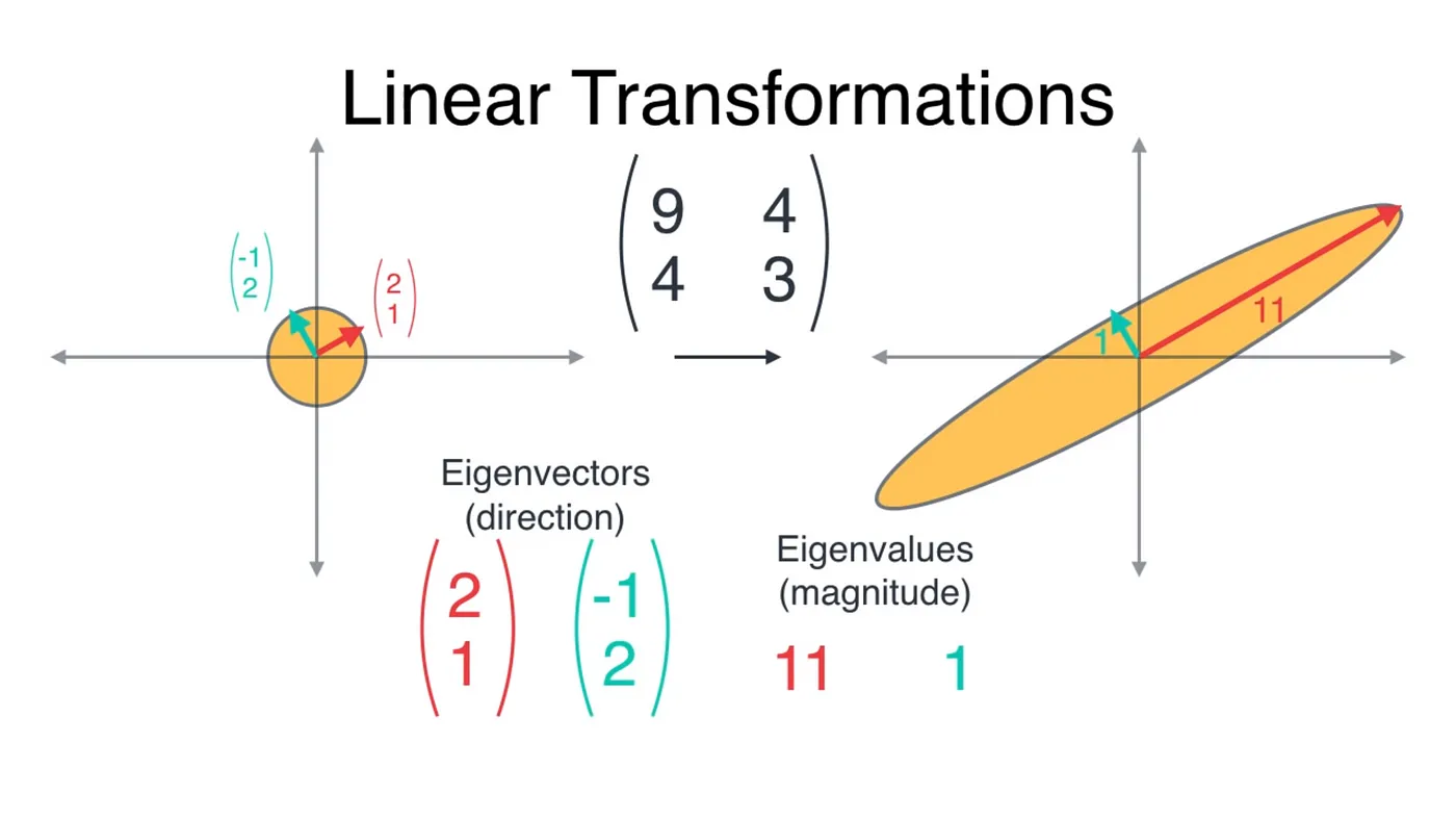
The question is: which eigenvector to choose?

Red is the better choice because it would retain maximum variance of the original dataset, which means maximum information is retained.

#The interesting part: code

We will apply the algorithm on word embeddings, which is a very high dimensional vector representation of, well, words. The TensorFlow visualization for 10,000 words in 200 dimensions is something like this:

We will use a dataset with embeddings in 300 dimensions instead.

The process is as follows:

1. Demean the data (center it, so each feature has zero mean);

def compute_pca(X, n_components=2):
    """
    Input:
        X: of dimension (m,n) where each row corresponds to a word vector
        n_components: Number of components you want to keep.
    Output:
        X_reduced: data transformed in 2 dims/columns + regenerated original data
    """
    # mean center the data (axis=0 because taking mean along columns)
    X_demeaned = X - np.mean(X, axis=0, keepdims=True) # normalize each feature of dataset

2. Compute the covariance matrix;

  # calculate the covariance matrix, rowvar=False because our features are in columns, not rows
    covariance_matrix = np.cov(X_demeaned, rowvar=False)

3. Compute and sort the eigenvectors and eigenvalues from highest to lowest magnitude (eigenvalues), remember we need high eigenvalue eigenvectors so as to retain maximum variance (information) of our word embeddings.

    # calculate eigenvectors & eigenvalues of the covariance matrix, both are returned in ascending order
    eigen_vals, eigen_vecs = np.linalg.eigh(covariance_matrix)
    # sort the eigen values (highest - lowest)
    eigen_vals_sorted = np.flip(eigen_vals)
    # sort eigenvectors (highest - lowest)
    eigen_vecs_sorted = np.flip(eigen_vecs, axis=1)

4. Select the n eigenvectors corresponding to the eigenvalues in descending order;

    # select the first n eigenvectors (n is desired dimension
    # of rescaled data array, or dims_rescaled_data), each      eigenvector is a column in eigen_vecs matrix.
    eigen_vecs_subset = eigen_vecs_sorted[:, :n_components]

5. Multiply this subset of eigenvectors by the demeaned data to get the transformed data.

   # transform the data by multiplying the demeaned dataset with the    first n eigenvectors
    X_reduced = np.dot(X_demeaned, eigen_vecs_subset)
    return X_reduced

#Let’s visualize!

words = ['oil', 'gas', 'happy', 'sad', 'city', 'town',
         'village', 'country', 'continent', 'petroleum', 'joyful'] #11 words
# given a list of words and the embeddings, it returns a matrix with all the embeddings
X = get_vectors(word_embeddings, words)
X.shape # returns (11, 300)
 
# We have done the plotting for you. Just run this cell.
result = compute_pca(X, 2)
plt.figure(figsize=(12,8))
plt.scatter(result[:, 0], result[:, 1])
for i, word in enumerate(words):
    plt.annotate(word, xy=(result[i, 0] - 0.05, result[i, 1] + 0.1), )
plt.show()

The output would be something like this:

Now we have reduced 300 dimension embeddings to 2 dimension embeddings! That is why we can visualize it!

I hope I explained everything is a friendly and easy manner :)

Note: All the illustrations shown in this article belong to a YouTube channel Luis Serrano. His video explaining PCA was amazing and here’s a link to his channel.

Osama Akhtar

Software Engineer

Written on Aug 5, 2020

Copy blog link